

Updated: August 2026.
If the hottest question about AI in 2023–2024 was “which model is better,” then starting in early 2026, the most costly question has shifted to: how much does it cost to run one token, and who runs it more cheaply. This is no longer a hardware question—anyone can buy a GPU. What now separates the winners from the losers is a very specific algorithmic layer between the model and the chip: how memory is organized, how tasks are scheduled, how to anticipate, and how to streamline operations.
What’s strange about 2026 is that API prices continue to fall while memory and GPUs are at record highs. Much of that discrepancy stems from the algorithms described below.
Root: a request with two phases and two opposing knots
To understand why a whole range of seemingly disparate techniques emerged at the same time, we must recognize a fundamental physical truth: text generation consists of two phases with completely different characteristics.
Prefill phase — the model reads the entire prompt. Since all tokens are loaded at once, the GPU can perform large-scale matrix multiplication and run at nearly full capacity: this is the computational bottleneck, where the cost increases with length, and the attention cost increases with the square of the length.
Decoding phase — a token-by-token generative model, where each token depends on the previous one, making parallelization impossible. Each step must re-read all active weights from HBM just to generate a single token: for a model with tens of billions of parameters, that amounts to tens of gigabytes read per token, while the actual computations required are minuscule. The result: on small batches, the GPU uses only a few percent of its computational capacity, with the rest of the time spent waiting for memory.
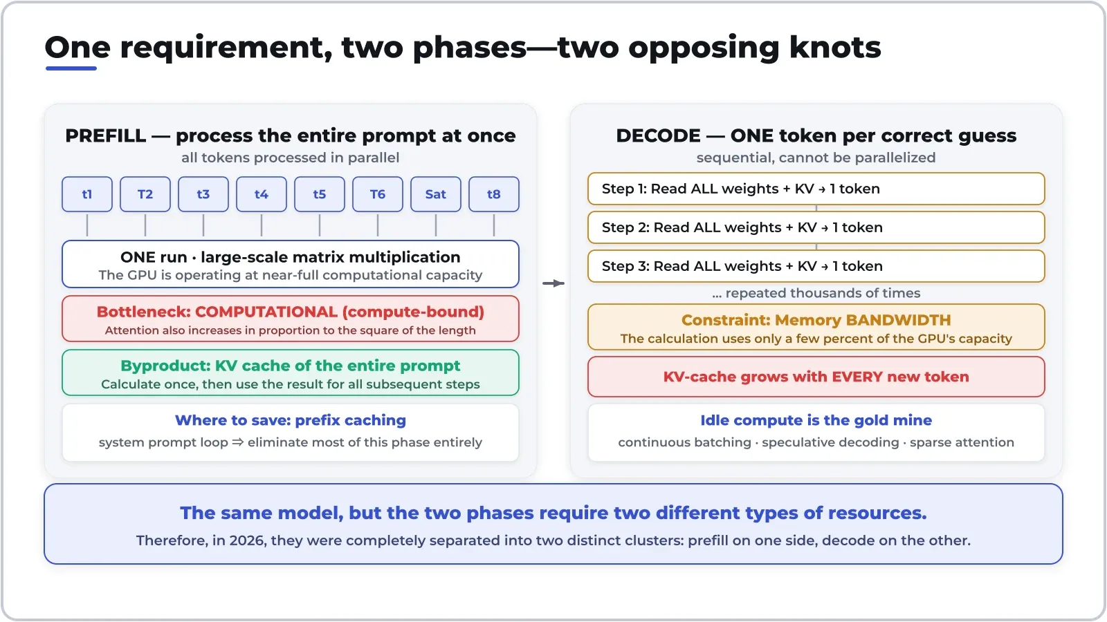
This entire article is essentially just a consequence of one statement: during the decoding phase, there is an excess of computation but a shortage of bandwidth. Every algorithm that accelerates inference is a way to reduce the excess in order to make up for the shortage.
KV-cache: When a model needs a small operating system
To avoid recalculating attention for the entire history at every step, the model retains the key and value vectors of every token that has passed through—this is the KV-cache, which turns long context into cash: each new token adds another piece, and that cache must reside in the HBM, competing for space with the weights themselves.
The naive approach is to allocate a contiguous block of memory large enough to accommodate the maximum length for each request—resulting in terrible fragmentation, with most of the memory reserved but unused. PagedAttention solves the problem exactly as an operating system solves the virtual memory problem: it divides the KV-cache into fixed-size blocks, maintains a mapping table from logical addresses to physical blocks, and allocates memory incrementally as needed. No contiguity is required, fragmentation is virtually nonexistent, and more importantly—if two requests share a common head, they share the same block, just like copy-on-write.
From that idea of chunking emerged the most cost-effective solution in practice: prefix caching. System prompts, tool descriptions, attached documents, conversation history—in real-world applications, repetitive content makes up the majority of the input. Hashing each block of content and looking it up in a table is enough to eliminate most of the prefill phase for subsequent calls. This is why major providers list separate prices for cached inputs, which are typically about one-tenth the cost. In other words: a data structure has become a separate line item on the price list.
By 2026, this cache will be tiered to server RAM and then to SSDs, and the router must know which machine holds the cache in order to route requests to that specific machine—even distribution-style load balancing has become the wrong choice, because sending a request to an idle machine without the cache is more expensive than queuing it on a machine that does have the cache.
Scheduling: Continuous batch merging and prefill splitting
Combining multiple requests into a single run helps share the cost of reading weights—read once, use for the entire batch. But the old-style batching (waiting for a full batch, running, then waiting for the entire batch to finish) is wasteful: short requests have to wait for long ones. Continuous batching schedules at the token-generation step level: as soon as a request finishes, it leaves the batch, and the empty slot is filled by a new request in the next step. Simply changing the scheduling granularity has increased throughput many times over on real-world workloads, without touching the model at all.
The remaining issue is two phases that overlap: a long prompt being prefilled takes up the GPU for hundreds of milliseconds, causing all requests currently being decoded to stall. Chunked prefill breaks the prefill process into smaller chunks interspersed with decoding steps, trading a bit of wait time for the first character for smoother performance across the board—blurring the line between algorithm and business policy.
Guess and then check: get rid of what you have too much of to buy what you’re missing
If decoding involves extra computations but lacks bandwidth, checking five tokens in a single pass is almost no more expensive than checking a single token—because both operations must read the same number of weights. That is the whole idea behind speculative decoding.
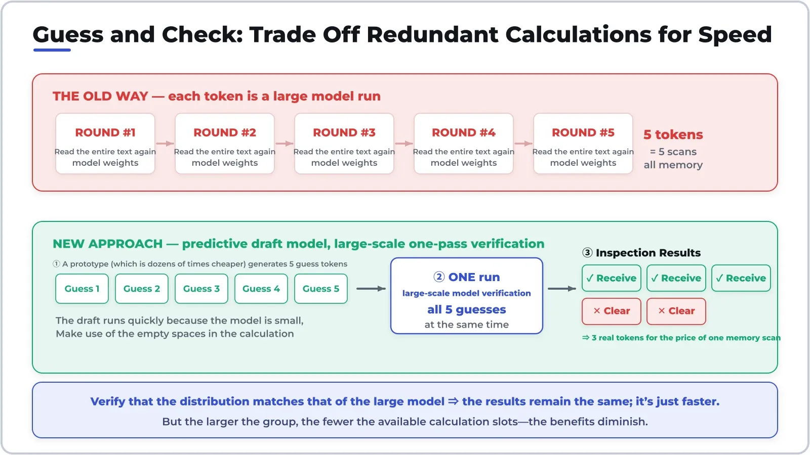
Mechanism: A low-cost draft model proposes the next few tokens; the large model runs a single pass to check the entire sequence; if a token matches, it is accepted; if the first token is off, it is discarded and regenerated. The most subtle aspect is the verification step, which uses adjusted sampling to ensure the output distribution is identical to that of a standard large-scale model run. This is not a quality-compromising approximation—which is why it is enabled by default without requiring any permission.
The trend for 2026 is to keep the prediction head separate: instead of training a separate small model, researchers directly attach a multi-token prediction head to the large model itself, or use a lightweight prediction head that reads the model’s internal state directly. The EAGLE-3 line and its multi-token prediction variants were merged into the main branches of vLLM, SGLang, and TensorRT-LLM early this year; the average number of tokens accepted per turn ranges from two to three.
But let’s be clear about the limitations: the benefits diminish as the batch size increases. The larger the batch, the closer the GPU gets to its computational capacity, leaving no room for over-prediction; the acceptance rate also drops when the context is very long. Therefore, this is a tool for reducing latency and for off-peak hours, not an unconditional solution for increasing throughput.
The Real Breakout of 2026: Pay Attention—Keep an Eye on Every Token
All of the above are operational optimizations: the model remains unchanged. The biggest change starting in early 2026 runs deeper—the architecture itself is being revised to prevent the KV-cache from continuing to grow. Three approaches are being pursued in parallel:
- Compress KV pairs into a latent state. Instead of storing the full keys and values for each attention head, project them onto a much smaller latent vector and then unpack them during computation—the multi-head latent attention approach reduces cache usage by a factor of many with virtually no loss in quality.
- Sparse attention is learnable. Each new token does not need to examine the entire history; a low-cost index selects a small set of relevant tokens, and attention is computed only on that set. Unlike the old-school “sliding window,” the selection here is trained alongside the model rather than being a hard rule set by the user.
- The most surprising innovation is the hybrid with linear-directional attention. Most layers are replaced by a gated regression variant, where each layer maintains a fixed-size state rather than an infinitely long cache, and a full attention layer is inserted every few layers to preserve accurate memory. The ratio of three linear layers to one full layer has appeared in many open-source model families in the first half of 2026.
The economic implications of the third approach are significant. With traditional attention, where the context is doubled, each decoding step must process twice as much information—the cost per token increases with the length of the conversation. With most of the model consisting of a fixed-state regression layer, the cost per token remains nearly constant regardless of length. Just as models and agents begin generating sessions hundreds of thousands of tokens long, that is the difference between having a business model and not having one.
One point that may not necessarily need to be mentioned: removing tokens to make the text easier to read always carries the risk of omitting an important token. Accurate recall tests in long contexts remain the area where these architectures are scrutinized most closely, and current measurement methods are not yet standardized.
Separate the machine into: prefill one cluster, decode one cluster
If two phases require two conflicting types of resources, confining them to the same machine forces both to compromise. By 2026, separating prefill from decode had become the default configuration at scale: one group of machines runs only prefill, generates the KV-cache, and then transfers it over a high-speed network to a group of machines running only decode. Each side selects its own parallel configuration and batch size, scaling independently based on the ratio of long-to-short prompts in the actual workload.
This is combined with large-scale expert parallelization for the MoE model. MoE activates only a small fraction of the parameters for each token, but if all experts share a few GPUs, there is still a significant amount of read traffic. By distributing the experts across dozens of GPUs connected via ultra-high-bandwidth links—such as the GB200/GB300 NVL72 rack—each GPU holds only a few experts, significantly reducing the amount of weight data read per token and increasing the throughput per GPU many times over compared to running on a single machine.
Economics Corner: The Four Numbers Behind the Price of Each Token
The cost of a token, put simply, is the hourly GPU rental fee divided by the number of tokens that GPU produces per hour. The numerator is determined by the hardware market and is already under pressure; the entire algorithmic layer above does nothing but push the denominator up—but it must maintain the latency commitment, because throughput gained by making users wait is unsellable. The industry calls this metric “goodput.” Four levers, ranked by profitability:
- Prefix cache hit rate — the cheapest and most overlooked. A stable system prompt that places the invariant portion at the beginning can eliminate most of the input cost without changing a single line of the model.
- Effective batch size. Larger batches distribute the cost of reading weights evenly, but require more KV-cache, which is limited in HBM. You should either reduce KV precision to FP8 or compress KVs using architecture—both are indirect ways to buy more batch size—which is why KV quantization belongs to the cost-reduction algorithm category rather than the data compression category.
- Number of tokens generated per run. Speculation suggests this number could be increased from one to two or three.
- The number of weights to read for each token. MoE combined with parallel, wide-area experts directly targets this—the lever with the greatest impact.
There is one consequence that few people notice: the inference model generates a large number of output tokens relative to the input, which shifts the cost focus from prefill to decode. This means that everything optimized for decode—bandwidth, small KV, speculation, MoE—is suddenly worth many times more than it was two years ago, while optimizing prefill has become less important. The infrastructure for 2026 is being redesigned around that shift.
Prediction
- Attention will once again become the default. By the end of 2026, most new open models will use a hybrid of linear/sparse layers and full attention layers; full attention throughout the entire model will become the exception, reserved only for small models or short contexts.
- Draft models will disappear from deployment profiles. Multi-token predictors will be trained and released with their weights as part of the model, rather than something operators must assemble themselves.
- Performance metrics shift from GPUs to racks. The comparable metric will be tokens per second per rack at a guaranteed latency level—since phase separation and large-scale parallelism only make sense when calculated across an entire cluster.
- Cache becomes a storage tier with its own pricing. A tiered prefix cache (HBM → RAM → SSD), shared across multiple machines, includes cache-aware routing; the API pricing continues to be broken down by cache state rather than a single input price.
- A minor reality check regarding metrics. The more systems reduce tokens to save resources, the more likely there will be significant debate about whether long-term context scores mask actual performance losses in precise retrieval tasks.
Key takeaway: Over the past two years, most of the cost reduction in AI has not come from new chips but from fewer memory accesses per token. All the algorithms listed above—paging, prefix caching, continuous batching, predict-and-check, sparse and linear attention, phase separation, and expert spreading—are simply different ways of expressing that same idea. Those who understand that the bottleneck lies in bandwidth rather than computation will optimize effectively; those who don’t will buy more GPUs and still pay a high price.
Thảo luận